

Autoencoders are a class of artificial neural networks in which the neural network is expected to recreate the input at the output layer (instead of making a prediction on the input data). While this might sound odd at first, such a network becomes interesting when the intermediate hidden layers have smaller dimension as compared to the input layer. Thus we end up learning the compressed or compacted representation of our input data. Hence, we successfully achieve our goal of dimensionality reduction. Moreever, a new input data point can be fed to this trained network and if the reconstruction error in the output exceeds certain threshold, we can say that the new data point was different from the class of input data and hence might as well be classified into different class/category or as an anomaly. The representation from the hidden layers of the network is sometimes referred to as the latent representation.
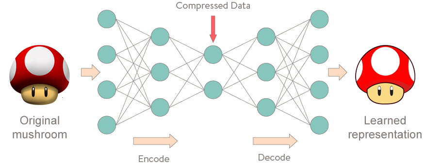
Let \( x \) be the input and \(\hat{x}\) be the reconstructed input (output). The objective function for a vanilla autoencoder looks something like below:
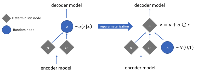
Variation Autoencoders (VAE) are special kind of autoencoders, that enable probabilistic inference. These networks, instead of learning a numerical value for each dimension of the latent state, rather learn a distribution.
The variational part here refers to the Variational Bayesian Methods, which are a family of techniques that allow us to re-write statistical inference problems (that involve inferring the value of a random varaible given value of another random variable) as optimization problems and vice versa. Leave a comment if you wish that I write a blog post on that. We use the objective for the simplest VB method viz. Variational lower bound or the mean field approximation.
The paper can be found here
Disclaimer: This post does not cover all of the paper, but merely one of the applications of it. The techniques in the paper are more widely applicable than just to variational autoencoders
While using autoencoder we could learn the deterministic/fixed value for each attribute/dimension in the latent representation of each data point, we may prefer to represent each latent dimension as a range of possible values. Ergo, given an input, we can now represent the latent state as a probability distribution. The decoder will then randomly sample from this distribution of latent state to generate an input vector for the decoder network. This also ensures that the close by values in the input space correspond to similar decodings for the decoder. Since the decoder now has a much larger set of values (as sampled from the latent state distribution), we can expect the decoder to be much more robust now and be able to better reconstruct the inputs belonging to similar classes as the training dataset.
Variational Autoencoders are like a blend of neural networks with the theory of probabilistic graphical models. Let us consider the following simple graphical model to arrive at the objective function of the autoencoder. We will then derive analogy between the graphical model and the variational autoencoder.
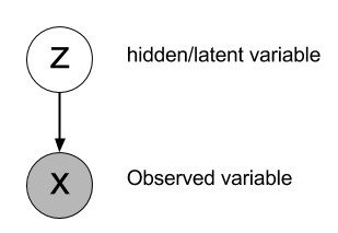
X is a random variable that is observed (or analogous to the input variable) while the random variable Z represents the latent or the hidden state. To compute the hidden state, we need \( P(Z|X) \)
By Bayes’ Theorem, we have:
where,
However, the problem above is complicated and often intractable to compute analytically. Also, sampling based methods like Markov Chain Monte Carlo can be extremely slow to converge. Read more about intractable posterior distributions. Hence we resort to variational inference.
The key idea is to approximate \( P(Z|X) \) with another distribution \( Q_{\phi}(Z|X) \) like a gaussian, for which we can easily perform posterior inference and adjust the parameters of Q such that it is close to P. To do this we use the reverse KL-divergence as a distance metric. Note that using reverse KL-divergence ensures that our Q is zero-forcing rather than zero-avoiding distribution.
With some simplification, we arrive at:
Telling us that minimizing KL is equivalent to maximzing the negative of the second term. With some more simplification to it we obtain:
L is therefore, expected decoding likelihood plus KL divergence between variational approximation and the prior on Z. To draw the analogy with our autoencoder, the encoding layer is represented by \( q(z|x) \) while the decoding layer by \(p(x|z)\). Our objective function thus will consist of the terms that maximize the reconstruction likelihood and that encourage the approximation to the true distribution to be as close to the true distribution as possible.
Variational Autoencoders end up learning much smoother latent space representations of the input data. These also form much more robust models for anomaly detection as they can more comfortably reconstruct any input point come whose latent space representation is somewhere in the areas where vanilla autoencoders had gap (no latent point representation) but is still not out of class. Also these models can be used as generative models to produce more data which is similar to the input data. Overall the whole idea of bringing in probabilistic graphical models into this space is very powerful as it introduces new possibilities that enables probabilitic inference of neural networks.
Some more reference material: