A brief summary of the infamous 'Attention Is All You Need'
While this paper has been around for a while now, it wasn’t until recently that I realized how terribly I needed to update my knowledge on the topic. And that happened only a few days ago when someone claimed that I was speaking gibberish talking about deep RNNs, LSTMs/GRUs and that many of those are now considered old school in dealing with several tasks.
So, what is all the fuss about?
This is an extremely influential paper, that came out of google brain in the late 2017
The authors introduced a Transformer model which is a simplistic model with a few matrix multiplication combined with a simple 2 layer feed forward network (or solely attention based model with no deep recurrent network)
And this model surpasses several of the SOTA models in their respective tasks by a good margin.
Hence the comic title and the surrounding fuss
Motivating non-RNN based architecture
The then SOTA RNN architectures suffered from the following problems:
difficult to parallelize
unable/difficult to capture long range dependencies (while LSTM try to capture certain long range dependencies, their idea of long is really not very long)
Transformer Architecture
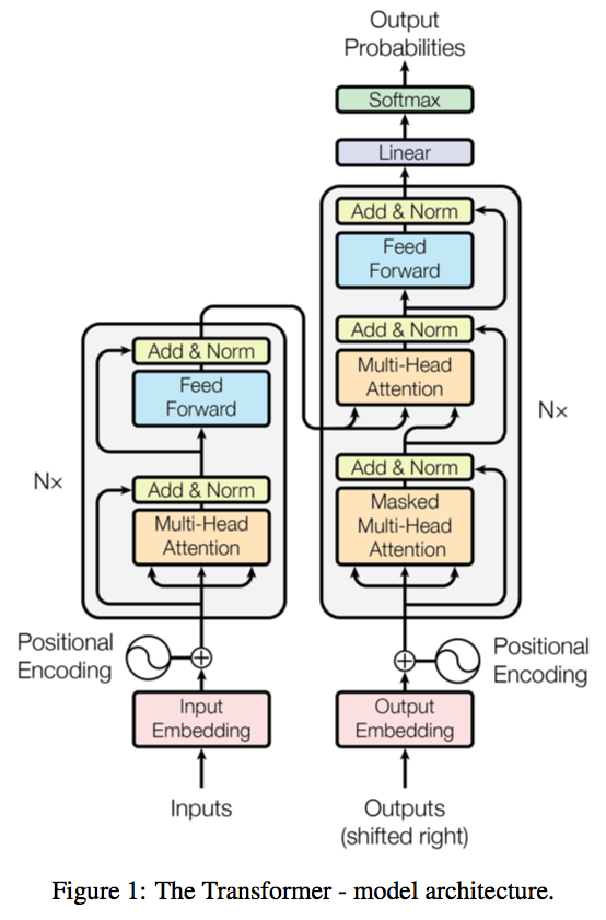
The transfomer uses stacked self-attention and point-wise, fully connected layers as shown in the figure above
The left-side network is known as encoder stack, while the right part is called the decoder stack
Encoder Stack:
Input Embeddings: Input words (represented as one-hot vectors) are first represented as word vectors using word embeddings. Dimension of each input embedding be dmodel
Position Embedding: The position embeddings (which have the same dimension dmodel) are then summed with the input embeddings. More details on this can be found below
Attention:
Given a set of key-value vector pairs K, V and a query vector Q, attention can be described as a weighted sum of vectors in V, where weight assigned to each value is computed by a compatibility function of the query with the corresponding key vectors
There are a few kinds of attention mechanisms named based on the way the compatibility of key with query is measured
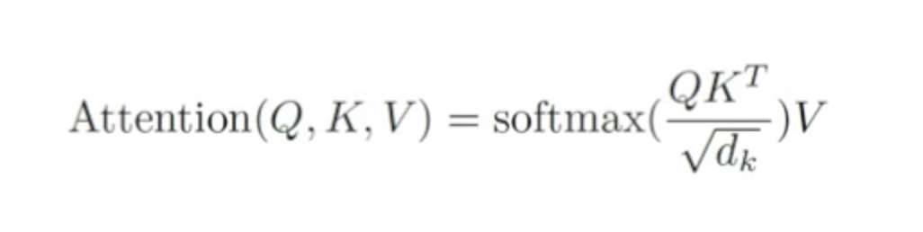
The one that is used in the paper is Scaled Dot-Product Attention, in which the compatibility of key k and query q is measured as the normalized/scaled dot product of k and q (which is then passed through softmax function). When multiple query vectors are packed together in a matrix Q, this can be represented as follows.
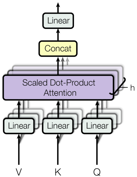
Multi-Head Attention:
Instead of performing the above step a single time, the self attention mechanism is applied h times on different linear projections of the keys, values and the queries, results from who are concatenated and undergo a linear projection once again to produce the final output as shown below.
Each linear projection in the above description sort of projects one part of the key, value and query vector out. Multi-head attention allows the model to jointly attend to information from different representation subspaces at different positions. With a single attention head, averaging inhibits this
The encoder contains self-attention layers. In a self-attention layer all of the keys, values and queries come from the same place. This sort of intuitively does the function adding information of words around sentence that might relate to this word.
Similarly, self-attention layers in the decoder allow each position in the decoder to attend toall positions in the decoder up to and including that position. (masking i.e. substituting -INF inplace of illegal values, or the values that are ahead of the current word, is done before taking softmax)
Finally, there standard “encoder-decoder attention” being used in the decoder stack, where the key-values are the output of encoder stack and the query vectors come from the decoder stack
Position-wise feed forward network: Finally, each of the encoder and decoder stack end with a fullyconnected feed-forward network, which is applied to each position separately. This contains a single hidden layer with ReLU activation and can be represented as: FFN(x) = max(0,xW1+b1)W2+b2
Position Embeddings:
Position embeddings are formed from sine and cosine functions of the different frequencies at each dimension
where pos is the position and i is the dimension
however, authors confirm that they received similar results with a few other kinds of position encodings too
While this is a slight technical detail from the paper, I would not worry too much about this since this is not where the actual meat lies
Intuition into why this approach maybe better
This can be viewed from three fronts:
Computational complexity: While RNNs take O(nd2), transformer requires O(n2d). When n < d, which is generally the case with most SOTA models, the proposed approach is computationally more attactive.
Amount of parallelization that can be acheived: Here, the current approach is clear winner. While layers in an RNN had to be executed sequentially and required O(n) sequential operation, here we can do all the computation during the training phase in just a few large matrix multiplication steps.
Path Length of long range dependencies: Here again, while the path length between long range dependncies was linear in an RNN and logarithmic in a stacked/heirarchial CNN, it is a single step in the current proposed approach.
All in all, the paper demonstrates how powerful tools at hand can be if the problem is modelled correctly. This hints at several other hidden modelling possibilities that might be waiting to be uncovered.